Note: The steps described in this article are based on Microsoft Excel 2007.

One of the uses of MS Excel is to easily and quickly create fill-in forms. A common feature in fill-in forms is the automation of field entries based on a list item selection. This article shows a simple way of how to create a drop-down list. The article than proceeds to show how cell values can be changed when the list item selected is changed.

Creating the drop-down list items

Creating a drop-down list is very easy. In this article we create the list in a separate worksheet from where the list will be used.

1. Open a new worksheet. You can either use one of the worksheets already created by Excel when creating a new document or by using the ‘New Tab’ button at the bottom of the screen (see Figure 1).
   
   

   Figure 1

2. In the newly created worksheet write the items under each other. Figure 2 shows an example of a list.
   
   

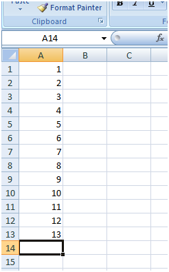
   Figure 2

3. The last step is to give a name to the list. To do this, highlight the list you created in point 2. Then in the Name Box (see Figure 3) type in the list name.
   
   

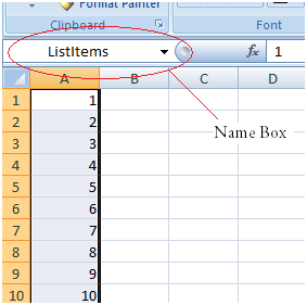
   Figure 3

   
   Note: For the purpose of this article the list name is set to ‘ListItems’

Creating the drop-down cell

1. Switch back to the worksheet where the form is beign creating
2. Select the cell that will be holding the drop-down list
3. From the Data menu click the ‘Data Validation’ button (see Figure 4). This will open the window shown in Figure 5.
   

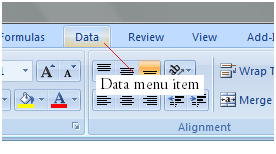
   Figure 4

   
   
   

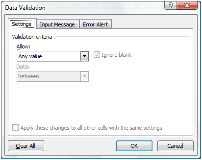
   Figure 5

4. Change the ‘Allow:’ drop-down value to ‘List’ (Figure 6)
   
   

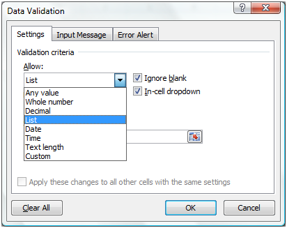
   Figure 6

5. Now a new field labelled ‘Source:’ has been added to the window. In the newly added field type ‘=<the name of the list>’. Continuing on this article’s example the field value is set to ‘=ListItems’ (see Figure 7). Then press Ok and the cell selected on point 2 is converted into a drop-down list (see Figure 8).
   
   

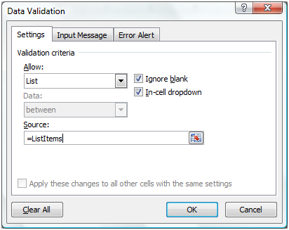
   Figure 7

   
   
   

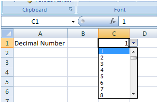
   Figure 8

Linking a cell to the drop-down value

Earlier in the article we have created a list of items which we used as a drop-down list. Now it is time to create the automatic insertion of contents in a cell based on the list selected item. There are two scenarios that one might have to handle:

1. The value of the drop-down cell needs to be copied into a new cell. This is an easy step as all that has to be done is to set the cell formula to ‘=<drop-down cell>’. If we had to do this in the article’s example the cell formula will be ‘=C1’.
2. A more complex scenario is when the value displayed in the cell is different from the drop-down select item. To handle this scenario further steps needs to be undertaken:
   1. Switch to the worksheet containing the list items.
   2. In the column next to the list items add their corresponding values to be used in the form cell (as shown in Figure 9).
      

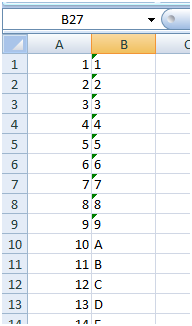
      Figure 9

   3. Switch back to the worksheet containing the form.
   4. Select the form cell that will contain the value associated with the selected drop-down item.
   5. Set the cell formula to

      =INDEX(<table with list items and their corresponding values>, 
      MATCH(<drop-down cell>, <List name>, 0), 
      <column index where the values to be used are located within the table passed as the first parameter)

      Where the ‘INDEX’ function instructs Excel to select the value in a specific row and column from an array that is specified in the 1st parameter. In the case of this article the column is the second column in the array, so the value for the parameter is set to 2. However determining the row number is not that simple. As the drop-down cell will only contain the list item text we need to determine the related row. To do this Excel provides the ‘MATCH’ function. The ‘MATCH’ function searches an array for a specific criterion and returns the index that satisfies the search criteria best.

Figure 10

This article showed a simple way of creating a drop-down list and how cell’s can be linked to the drop-down list value.
Article sample file: How to link a cell value with a an Excel drop down list

References

• Microsoft Office: Create a drop down list from a range of cells
• Microsoft Knowledge Base: How to use the INDEX and MATCH worksheet functions with multiple criteria in Excel