Hi, in this blog we take a look how we can highlight a set of rows in Microsoft Excel that fall between two dates.  This is inspired from Rodel Balasabas comment in my other post about highlighting a row in Excel. Thanks!

The final product looks as:

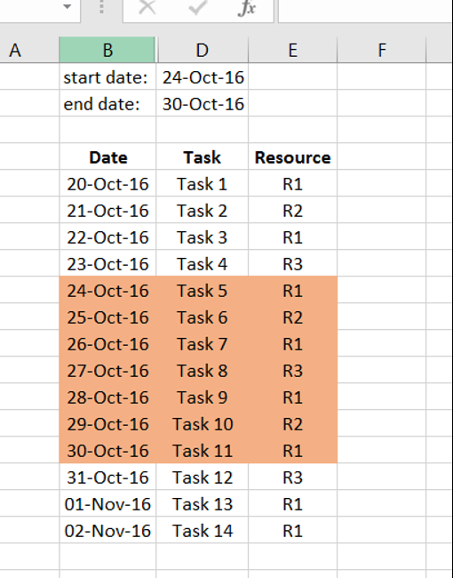
Final product

Adding multiple conditions to Excel’s conditional format may prove difficult if not impossible at times.  Thus, one trick is to add a hidden column in your table that does all your conditional logic and then use the result of this formula to highlight your rows.  The screenshot below shows all the formulas in our sheet.

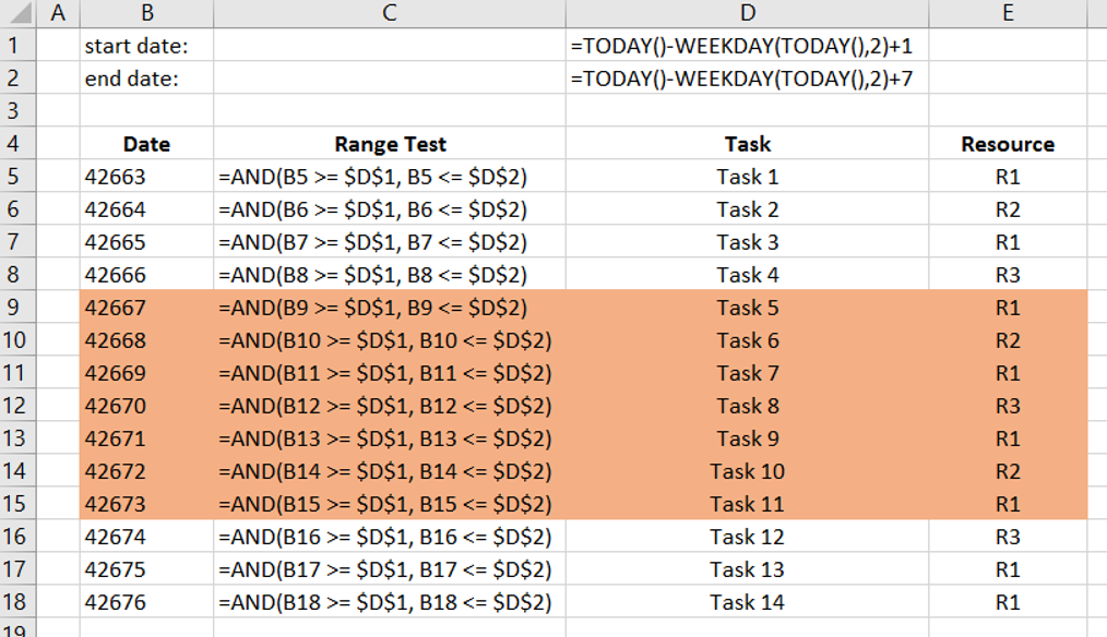
Sheet formulas

Let’s see how we can do this together.

Step 1

Put your data in a table:

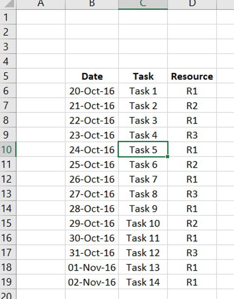
Our data

Step 2

Create week start date and end date.  We will use formulas so that these are automatically updated every week.

The formula for start of week (starting on a Monday) is: =TODAY()-WEEKDAY(TODAY(),2)+1

The formula for end of week is: =TODAY()-WEEKDAY(TODAY(),2)+7

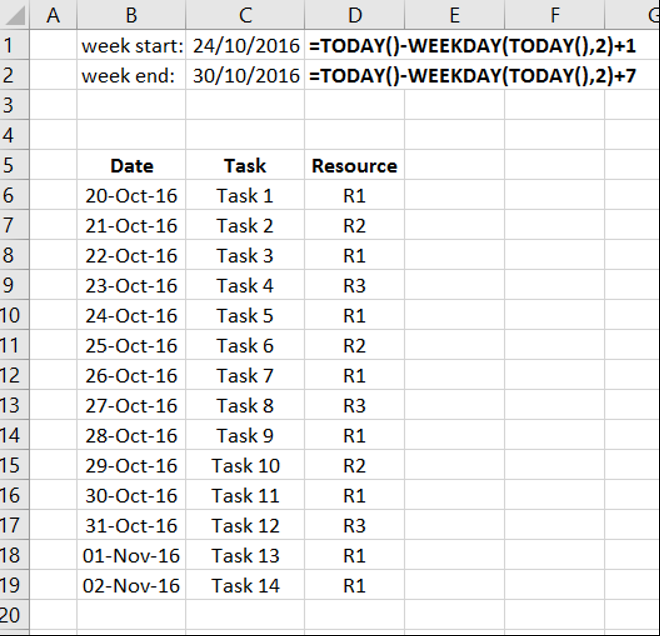
Adding start and end dates of current week.

Step 3

Add a column so that it evaluates to whether the date we have in our schedule is between our start and end dates.  To do this, we will use a simple AND() function to check if the date at hand is greater or equal to the start of the week and less or equal to the end date of the week.  A typical formula for such logic is =AND(B5 >= $D$1, B5 <= $D$2).

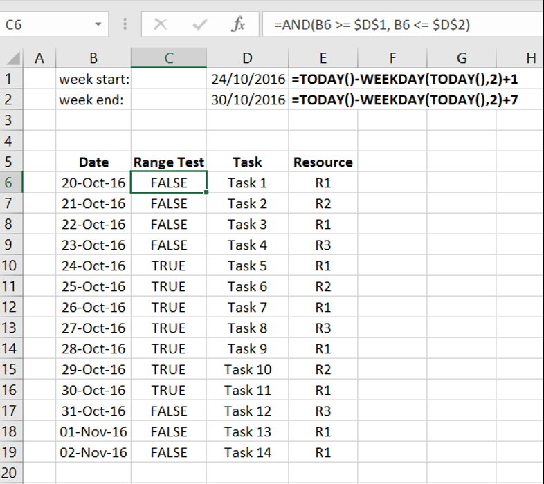
Adding logic that later will be used to indicate whether to highlight a row or not.

Step 4

Now we can hide our test column and create a new formatting rule based on column C.  The formula for this rule will be =INDIRECT(“C”&ROW()).  For more details how to do this see other blog post Highlight a row in Excel based on a cell value.

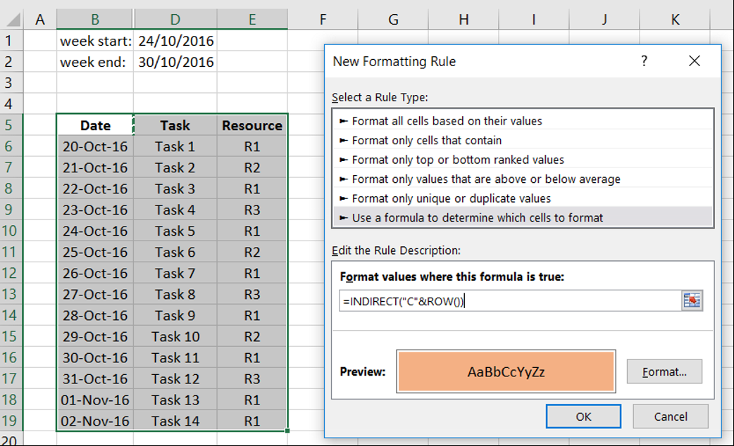
Adding cell formatting.

Once we hit the OK button, our table rows that falls in the range specified before will be highlighted.

I hope that you find this blog post useful.  If so, please leave us a message.

Thanks!